Methodology

Requirements

To carry out this project the following were needed:

1. LandSat satellite Imagery of Path 19/31 on the required dates ie July 16, 2002 and August 01, 2002

2. In-situ data for the same dates

3. Image processing software

LandSat imagery was acquired from Ohioview on the required dates ie., August 1, 2002 (Path 19/31), August 8, 2002(Path 20/31) and July 16, 2002(Path 19/31). The in-situ turbidity data was acquired from the University of Toledo for the above dates. ENVI 3.4 was chosen for image processing as it had some useful functions built into it i.e. BandMath etc. A methodology (Fig.3) was developed before executing the project in order to approach the problem in a mannered way.

Regression Model

Striped Right Arrow: Extracted Values from pixels
turbidity values from data

Step 5

Step 4

Step 3

Step 1

Step 2

Flowchart: Process: Creating a Shapefile
Using ArcView Flowchart: Process: Boat Data
Acquired from U.Toledo Flowchart: Process: Landsat Images
Acquired from OhioView Oval: Overlaying of point data onto Image and applying BandMath

And LandsatImage Flowchart: Process: Preprocessing Images
Dark object subtraction etc

Assumptions

Overlay of boat data and Raster data

Now going through step by step process........

Step 1

Collection of data:

The required data ie boat data and cloud free LandSat Imagery were acquired

Step 2

Assumptions:

1. The atmospheric conditions were assumed to be the same during the boat data collection and satellite overpass

2.The wind direction and water current conditions are assumed to be same during the satellite overpass and data collection

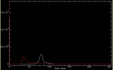
Dark Object Subtraction:

Examine brightness values in an area of shadow or for a very dark object (such as a large clear lake) and determine the minimum value. The correction is applied by subtracting the minimum observed value, determined for each specific band, from all pixel values in each respective band. Since scattering is wavelength dependent the minimum values will vary from band to band. 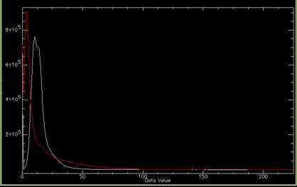This method is based on the assumption that the reflectance from these features, if the atmosphere is clear, should be very small, if not zero. A histogram after dark object subtraction for the same image can be seen in the Fig.5 below.

Fig. 4 showing the digital numbers of band 3 and 1 of LandSat before Dark Object Subtraction

Fig.5 showing the digital numbers of band 3 and 1 of LandSat after Dark Object Subtraction

Fig.8 (August 1, 2002)

Spatial and spectral subset:

Spatial and spectral subset were made to the dark object subtracted images. The image is subset spatially and spectrally to decrease the processing time and memory. It was found out empirically that Band 3 and Band 1 of LandSat ETM are closely related with turbidity values (refer Fig.6). Hence the images were spectrally subset for bands 1 and band 3.The processed images could be seen in figures 7, 8&9 below.

Step 3

Preprocessing of the images:

The images acquired were first preprocessed using some of the basic tools in ENVI 3.5. Dark Object Subtraction was applied to the images. The atmosphere introduces two forms of path radiance into the signal, radiance from Rayleigh or molecular scatter, and radiance from aerosols or haze. These can be removed simultaneously using dark object subtractions (refer Fig 4).

Boat data:

The in-situ boat data was collected in the western basin of Lake Erie at 28 points on two dates i.e.., July 16, 2002 and Aug 1, 2002. The data includes the sechhi depth measurements converted to NTU (Nephelometric Turbidity Unit). The points have longitude and latitude collected with a GPS unit. The data is added to ArcView 3.3 to create a point shapefile with the 28 points of in-situ measurements. The point layer is then projected to the coordinates of the image i.e.., NAD 1983 datum.

Step 4:

The file is then brought into ENVI3.5 and was overlaid onto the preprocessed image (refer fig 10 & 11).

Fig.7(July 16, 2002)

Fig.6 Reflectance curves of LandSat 7 ETM⁺ Bands 3 and 1 .Click on the image to see a detailed picture

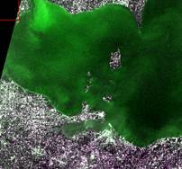
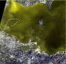
Fig.10 Point data overlayed onto preprocessed LandSat 7 ETM⁺ image of July 16, 2002

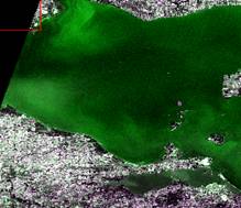
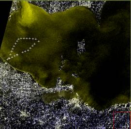
Fig.11 Point data overlayed onto preprocessed LandSat 7 ETM⁺ image of August 1, 2002

Step 5:

Brightness values were extracted from the satellite digital data and were used to develop regression models with in-situ sampling . Linear regression models were developed from brightness values and onsite sampling data. Data from the 28 individual sampling sites were compared with the average brightness of the red (band3) and blue (band1) reflectance of water and turbidity. Histograms and tests of normality indicated the distributions of satellite sensor data were normal for the study area. a band math function was developed using the prior empirical functions derived by Czajkowski et al. The in-situ data was overlaid onto the images after reprojecting the point data into UTM (NAD 1983)and a new empirical model was developed using BandMath function in the image processing software ENVI 3.5 and was applied to the band ratio 3/1. An average of 9 pixels i.e. 3x3 matrix from BandMath applied LandSat image (each pixel is 30X30 mt) was taken as mean value for each of the 28 in-situ observations. Mean averages for all the 28 observations were taken. Regression analysis was applied to the data. The mean values with negative numbers were assumed to be that of clear waters and thus were not considered when running the analysis. After the analysis the BandMath processed images are made into turbidity maps reflecting the clarity of water. Fig 12 and Fig 13 represent the two turbidity maps i.e. July 16, 2002 and Aug 01, 2002. The darker tones represent more turbidity and the lighter tones represent low turbidity.

Fig.12 Turbidity map of July 16, 2002 showing the turbidity. Darker tone represents more turbid waters

Fig.13 Turbidity map of Aig 01, 2002 showing the turbidity. Darker tone represents more turbid waters

Introduction | Methodology | Results | Conclusions | References